2020-11-01

RobWorkStudio + ROS plugin template

I sometimes use RobWorkStudio to visualize the scene, robots, trajectories, and for the task interface. It's a nice tool to gather everything in the same place. This often requires enabling some ROS interaction, and it's not terribly straightforward to configure the build system for both ROS and RWS.

In this repository you can find a blank ROS package template containing a RWS plugin: RWS ROS plugin template.

Simply place the package in your catkin workspace and use catkin build or catkin_make to build it. It obviously requires RobWorkStudio to be installed and the environment variables RW_ROOT and RWS_ROOT pointing to RobWork package and RobWorkStudio package respectively. Please check the previous post to see how to do it.

The plugin template shows how to set up the build system and how to embed ROS node handle, subscribing and publishing in the plugin code. A sample subscriber listens to a /level [std_msgs/Int32] topic and updates a QT label in the GUI with the received data. A sample publisher outputs the data from a QSpinBox widget to a /measured [std_msgs/Int32] topic.

2020-10-31

RobWorkStudio plugin template

I haven't posted in a while. Let's start again with something small.

Whenever I have to create a new plugin for RWS, I find myself scavenging the source code from one of my older projects. I have to remove the excess bits, rename and edit the files and classes.

This is a repository containing a blank RWS plugin that you can use: RWS plugin template.

It contains a blank Qt UI file (with a test button added), CMake configuration and boilerplate source files.


This is how to use it:

1. Make sure you have your RobWork installed.

2. Configure the paths in your evironment. I recommend adding the following to your .bashrc:

export RW_ROOT=${HOME}/robwork/RobWork

export RWS_ROOT=${HOME}/robwork/RobWorkStudio

export RWSIM_ROOT=${HOME}/robwork/RobWorkSim

3. Download the repository, navigate to the build directory and execute build commands:

cmake ..

make

4. You should now have your plugin .so in the libs directory. You can add it in the RWS environment through the menu or append the following to the [Plugins] section in the RobWorkStudio.ini file:

RWSPluginTemplate\DockArea=2

RWSPluginTemplate\Filename=librws_plugin_template.so

RWSPluginTemplate\Path=<plugin path>/libs

RWSPluginTemplate\Visible=true

(You can change RWSPluginTemplate to whatever you want; do also change the file name and the path.)


You may want to edit the plugin naming before building it. You should change the following things:

1. Change .cpp, .hpp, and .ui file names.

2. In .cpp and .hpp files change the class name globally.

3. In .ui file change the widget name.

4. Update CMakeLists.txt with these names.

5. Add includes and libraries in CMakeLists.txt as necessary.

6. In plugin.json update the name field.

7. Test whether build still works after these modifications.


The plugin contains an example of how to service a push button and how to do some minor things with the workcell. Have fun.

2020-01-26

Simulating a drone in Gazebo part 2 - Gazebo plugin

Last time we have built a URDF model of a drone and spawned it in Gazebo. Today we will make a Gazebo plugin to control the drone.

Our goal is to create a Gazebo Model Plugin that will interface with ROS and add forces to the model based on the desired motor speeds, such that the drone will be able to fly. This is the very basic level of control, which we need to implement.

The plugin ROS interface will be as follows:
  • Drone pose in the world frame of reference will be published on the /pose topic. We will create a kair_drone/Pose message type for easy orientation representation using RPY angles.
  • The plugin will also publish the frame pose using a TF broadcaster on the /tf topic.
  • The plugin will listen for the kair_drone/MotorSpeed message on the /motor_speeds_cmd topic and apply the simulated forces to the model.
  • The plugin parameters will be defined as the SDF elements in the xacro model file.

As usual, the code is all available in the repository.

1. Creating the messages

First, we shall create the two message types necessary. The Pose message shall carry the complete position and orientation information about the model in simulation and the MotorSpeed will define the desired speeds for the six motors of the model.

The Pose message is defined in the msg/Pose.msg file as follows:

float32 x
float32 y
float32 z
float32 roll
float32 pitch
float32 yaw

 
There are several message types defined in the standard geometry_msgs package that we could use instead, e.g. Pose or Transform. These involve the conventional ROS quaternion representation though and it will be easier for us to represent the orientation as RPY angles explicitly.

The MotorSpeed message is defined in the msg/MotorSpeed.msg file:

string[] name
float32[] velocity

Next, we have to modify the CMakeLists.txt and the package.xml to enable message building. Make sure that the package has the following dependencies:
  • geometry_msgs
  • sensor_msgs
  • std_msgs
  • tf
  • message_generation
Next, make sure that the message definition and message generation sections in the CMakeLists.txt look like this:

## Generate messages in the 'msg' folder
add_message_files(
  FILES
  Pose.msg
  MotorSpeed.msg
)

## Generate added messages and services with any dependencies listed here
generate_messages(
  DEPENDENCIES
  geometry_msgs
  sensor_msgs
  std_msgs
)

Rebuild the project now and re-source the setup files:
cd ~/catkin_ws
catkin build
source devel/setup.bash

2. Preparing the build system for the Gazebo plugin

 The following changes need to be made to the CMakeLists.txt in order to build the Gazebo plugin:

  • in the system dependencies section:
## System dependencies are found with CMake's conventions
# find_package(Boost REQUIRED COMPONENTS system)
find_package(gazebo REQUIRED)

  • in the Build section:
## Specify additional locations of header files
## Your package locations should be listed before other locations
include_directories(
# include
  ${catkin_INCLUDE_DIRS}
  ${GAZEBO_INCLUDE_DIRS}
)

link_directories(
  ${GAZEBO_LIBRARY_DIRS}
)
list(APPEND CMAKE_CXX_FLAGS "${GAZEBO_CXX_FLAGS}")

  • and finally, we add the plugin target:
add_library(drone_plugin SHARED src/drone_plugin.cpp)
target_link_libraries(drone_plugin ${GAZEBO_LIBRARIES} ${catkin_LIBRARIES})

3. Creating the plugin

Let's begin by creating the boilerplate Model plugin file src/drone_plugin.cpp:

#include <iostream>
#include <gazebo/gazebo.hh>
#include <gazebo/physics/physics.hh>
#include <gazebo/common/common.hh>

class DronePlugin : public gazebo::ModelPlugin {
public:
  DronePlugin() : gazebo::ModelPlugin() {
    std::cout << "Starting drone_plugin" << std::endl;
  }
 
  virtual ~DronePlugin() {
    std::cout << "Closing drone_plugin" << std::endl;
  }

  void Load(gazebo::physics::ModelPtr parent, sdf::ElementPtr sdf) {
    _model = parent;
  }
 
private:
  gazebo::physics::ModelPtr _model;

};
 
GZ_REGISTER_MODEL_PLUGIN(DronePlugin)

This is the very basic plugin file structure that we will gradually expand. It is a good idea at this point to check whether the build system is set up properly:

cd ~/catkin_ws
catkin build

4. Reading the plugin parameters from SDF

If we want to specify the plugin parameters in the model SDF (and we do), we can then read them inside the plugin's Load() function. We will read the updateRate parameter (how often the pose messages shall be published), publishTf parameter (whether to publish the pose on /tf as well), rotorThrustCoeff (a coefficient that relates the rotor lift to its rotational speed) and rotorTorqueCoeff (which relates the rotor torque to its speed). This can be done by modifying the Load() function as:

  void Load(gazebo::physics::ModelPtr parent, sdf::ElementPtr sdf) {
    _model = parent;
   
    if (sdf->HasElement("updateRate")) {
      _rate = sdf->GetElement("updateRate")->Get<double>();
    } else {
      _rate = 100.0;
    }
   
    if (sdf->HasElement("publishTf")) {
      _publish_tf = sdf->GetElement("publishTf")->Get<bool>();
    } else {
      _publish_tf = true;
    }
   
    if (sdf->HasElement("rotorThrustCoeff")) {
      _rotor_thrust_coeff =
         sdf->GetElement("rotorThrustCoeff")->Get<double>();
    } else {
      _rotor_thrust_coeff = 0.00025;
    }
   
    if (sdf->HasElement("rotorTorqueCoeff")) {
      _rotor_torque_coeff =
        sdf->GetElement("rotorTorqueCoeff")->Get<double>();
    } else {
      _rotor_torque_coeff = 0.0000074;
    }

  }

Of course, the new variables also have to be added to the private section of the DronePlugin class:

private:
  double _rate;
  bool _publish_tf;
  double _rotor_thrust_coeff;
  double _rotor_torque_coeff;

5. Creating the ROS node

In order to enable the ROS interface, we need to create a ROS node handle during the plugin initialization. This is also done in the Load() function:

void Load(gazebo::physics::ModelPtr parent, sdf::ElementPtr sdf) {
  ...
 
  if (!ros::isInitialized()) {
    int argc = 0;
    char** argv = NULL;
    ros::init(argc, argv, "kair_drone",
       ros::init_options::NoSigintHandler);
  }

  _nh = new ros::NodeHandle("");
  _pose_pub = _nh->advertise<kair_drone::Pose>("pose", 100);
  _cmd_sub = _nh->subscribe("motor_speed_cmd", 100,
      &DronePlugin::onMotorSpeedsMsg, this);
  _ros_thread = 
      std::thread(std::bind(&DronePlugin::rosThread, this));
 
}

It is necessary to check whether the ROS was already initialized. Since we are going to launch Gazebo through gazebo_ros, it most likely was. We create a new ROS handle _nh and the /pose publisher and the /motor_speed_cmd subscriber as well. Furthermore, we also create a separate thread for ROS to spin in.

The onMotorSpeedsMsg() callback looks simple enough:

void onMotorSpeedsMsg(const kair_drone::MotorSpeed::ConstPtr& msg) {
  _cmd_mtx.lock();
  _motor_speed_msg = *msg;
  _cmd_mtx.unlock();
}

The rosThread() is the place where the ROS gets updated and where we will publish the model pose from:

void rosThread() {
  ros::Rate rate(_rate);
  while (ros::ok()) {
    ros::spinOnce();
    publishDronePose();
    rate.sleep();
  }
}

We might as well define the publishDronePose() method now:

void publishDronePose() {
  _pose_mtx.lock();
  gazebo::math::Pose pose = _pose;
  _pose_mtx.unlock();
 
  gazebo::math::Vector3 rpy = pose.rot.GetAsEuler();
  tf::Quaternion q(pose.rot.x, pose.rot.y, pose.rot.z, pose.rot.w);
  tf::Matrix3x3 m(q);
  double roll, pitch, yaw;
  m.getRPY(roll, pitch, yaw);
 
  kair_drone::Pose pose_msg;
  pose_msg.x = pose.pos.x;
  pose_msg.y = pose.pos.y;
  pose_msg.z = pose.pos.z;
  pose_msg.roll = roll;
  pose_msg.pitch = -pitch;
  pose_msg.yaw = yaw;
  _pose_pub.publish(pose_msg);
 
  if (_publish_tf) {
    tf::Transform T;
    T.setOrigin(tf::Vector3(pose.pos.x, pose.pos.y, pose.pos.z));
    T.setRotation(
      tf::Quaternion(pose.rot.x, pose.rot.y, 
        pose.rot.z, pose.rot.w));
    _tf.sendTransform(
        tf::StampedTransform(T, ros::Time::now(),
        "world", "drone"));
  }
}

Here you can see how the conversion from the conventional quaternion orientation to RPY is done. Notice also that we multiply pitch by -1. This is done in order to match the frame orientation in simulation with the common aircraft convention where the Z axis is expected to be directed downwards.

Please consult the complete code in the repository to see which headers and what data fields need to be added to the source at this point.

6. Adding the forces

The idea behind simulating the rotor equipped drone model is that at each step of the simulation we add an array of forces and torques to the drone body that correspond to the forces that would be exerted by the propellers (see Fig. 1). 
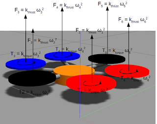
Fig. 1. Adding forces and torques to the model.

The forces for each of the propellers are calculated as:


The sgn() function is there to make it possible to define the direction of the torque by specifying the sign of the angular speed of the rotor.

Let us begin by adding yet another callback in the Load() function. This will make the onUpdate() method called at each step of the simulation:

void Load(gazebo::physics::ModelPtr parent, sdf::ElementPtr sdf) {
  ...
 
  _updateConnection =
      gazebo::event::Events::ConnectWorldUpdateBegin(
          std::bind(&DronePlugin::onUpdate, this));
}

The onUpdate() function updates the _pose (so only now will the publishDronePose work properly), and calls the updateThrust() method:

void onUpdate() {
  _pose_mtx.lock();
  _pose = _model->GetWorldPose();
  _pose_mtx.unlock();
 
  updateThrust();
}

The updateThrust() method looks up the child links of the model (so that is why we have modelled them as separate links attached by the revolute joints!) according to the name field in the MotorSpeed message, calculates the force and torque for each, and applies those to the link:

void updateThrust() {
  _cmd_mtx.lock();
  kair_drone::MotorSpeed cmd = _motor_speed_msg;
  _cmd_mtx.unlock();
 
  int n = cmd.name.size();
  for (int i = 0; i < n; ++i) {
    double thrust = calculateThrust(cmd.velocity[i]);
    double torque = calculateTorque(cmd.velocity[i]);
    gazebo::physics::LinkPtr link = _model->GetLink(cmd.name[i]);
    if (link != NULL) {
      link->AddLinkForce(gazebo::math::Vector3(0, 0, thrust));
      link->AddRelativeTorque(gazebo::math::Vector3(0, 0, torque));
    }
  }
}

 
AddLinkForce() and AddRelativeTorque() are the appropriate Gazebo methods to use here. The Gazebo documentation is sometimes quite insufficient in this regard, but these methods apply the force and torque respectively as an impulse; just in that one step of the simulation. What remains now is to calculate the force and torque for each of the propellers:

double calculateThrust(double w) {
  double thrust = _rotor_thrust_coeff * w * w;
  return thrust;
}

double calculateTorque(double w) {
  double torque = copysign(_rotor_torque_coeff * w * w, w);
  return torque;
}

7. Adding the plugin to the drone model

We can build the plugin now and add it to the drone model defined in urdf/drone.urdf.xacro. It goes right towards the end of the file:

...
<gazebo>
    <plugin name="drone_plugin" filename="libdrone_plugin.so">
      <updateRate>100</updateRate>
      <publishTf>true</publishTf>
      <rotorThrustCoeff>0.00025</rotorThrustCoeff>
      <rotorTorqueCoeff>0.0000074</rotorTorqueCoeff>
    </plugin>
  </gazebo>
</robot>

When we launch the program now:

roslaunch kair_drone gazebo.launch

we should see the /pose and /motor_speed_cmd visible in rostopic list. And we can now watch the drone fly (uncontrollably) up (Fig. 2)!

rostopic pub /motor_speed_cmd kair_drone/MotorSpeed "name: ['propeller1', 'propeller2', 'propeller3', 'propeller4', 'propeller5', 'propeller6']
velocity: [125, -125, 125, -125, 125, -125]" -1
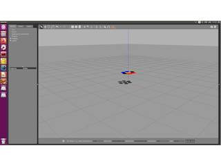
Fig. 2. Drone flying up!

2020-01-19

Simulating a drone in Gazebo

I wanted to test a certain thing in simulation and so I thought I'd prepare a drone model in Gazebo along with a simple autopilot. There is of course multiple existing frameworks (for example PixHawk already has Gazebo simulation: https://dev.px4.io/v1.9.0/en/simulation/gazebo.html), but I wanted something lightweight, and pretty much enjoy creating something from scratch. I'll describe the project in a series of posts. Today, we will build a simple URDF model of a hexacopter (see Fig. 1) and prepare the ROS package for further development.
Fig. 1. Simple drone model.


I've used the following software versions:
  • Ubuntu 16.04.3 LTS
  • ROS Kinetic 1.12.14
  • Gazebo 7.16.0
  • Python 2.7.12
... but it will probably work on the newer versions as well (let me know if anything needs updating!).

You can find the code for the whole tutorial on Gitlab HERE

1. Creating the package

Let's start with the package structure. Assuming you already have your catkin workspace configured (furthermore assuming it's located in ~/catkin_ws), let's create the package:

cd ~/catkin_ws/src
catkin_create_pkg kair_drone roscpp rospy std_msgs geometry_msgs sensor_msgs tf message_generation

This takes care of several dependencies we may use. We will add more of those later. Next, let's create a few directories:

cd drone
mkdir urdf launch rviz world

2. Creating the RVIZ launch file

When building an URDF model in a ROS package, it's usually a good idea to start with a launch file that will run RVIZ and upload the model to be visualized for you. Let's create the following rviz.launch file in the launch directory:

<launch>
  <!-- this defines the path to the URDF model -->
  <arg name="model" default="$(find kair_drone)/urdf/drone.urdf.xacro"/>

  <!-- this is the path to the rviz configuration file -->
  <arg name="rvizconfig" default="$(find kair_drone)/rviz/drone.rviz" />


  <!-- load the drone description onto the ROS parameter server -->
  <param name="robot_description" command="$(find xacro)/xacro --inorder $(arg model)"/>


  <!-- launch joint_state_publisher to publish fake joint states -->
  <node name="joint_state_publisher" pkg="joint_state_publisher" type="joint_state_publisher"/>


  <!-- launch robot_state_publisher to publish link positions -->
  <node name="robot_state_publisher" pkg="robot_state_publisher" type="state_publisher"/>

   <!-- launch rviz -->
  <node name="rviz" pkg="rviz" type="rviz" args="-d $(arg rvizconfig)" required="true"/>
</launch>


The model file and the rviz configuration file don't yet exist, so we will have to create those before launching RVIZ.


3. Building the hexacopter model

I opted for building the hexacopter model out of geometric primitives rather than molding the whole mesh in something like Blender. Since the hexacopter is highly symmetrical and has several repeating parts (arms, propellers), it's advisable to use XACRO to build the model. The listings below are a part of the drone.urdf.xacro file, which should be placed in the urdf directory of the package.

First, let us define some properties. You can change these if you wish to modify the drone overall shape.

<?xml version="1.0"?>
<robot xmlns:xacro="http://wiki.ros.org/xacro" name="drone">
 
  <!-- properties -->
  <xacro:property name="frame_radius" value="0.1"/>
  <xacro:property name="frame_height" value="0.05"/>
  <xacro:property name="frame_mass" value="0.88"/>
  <xacro:property name="arm_radius" value="0.01"/>
  <xacro:property name="arm_length" value="0.15"/>
  <xacro:property name="arm_mass" value="0.01"/>
  <xacro:property name="propeller_radius" value="0.1"/>
  <xacro:property name="propeller_height" value="0.01"/>
  <xacro:property name="propeller_height_offset" value="0.025"/>
  <xacro:property name="propeller_mass" value="0.01"/>


Next, we define a macro for calculating the inertia matrix for cylinder shapes (the whole model will be built out of cylinders).

   <xacro:macro name="cylinder_inertial" params="radius height mass *origin">
    <inertial>
      <mass value="${mass}"/>
      <xacro:insert_block name="origin"/>
      <inertia
        ixx="${0.0833333 * mass * (3 * radius * radius + height * height)}"
        ixy="0.0"
        ixz="0.0"
        iyy="${0.0833333 * mass * (3 * radius * radius + height * height)}"
        iyz="0.0"
        izz="${0.5 * mass * radius * radius}"
      />
    </inertial>
  </xacro:macro>


Since the model contains six arms, let us also create a macro for each of the arms. Note that we use expressions to calculate the positions of the arms around the drone frame. If you'd like your model to have fewer or more arms, you would have to modify these. The macro defines the arm link and the joint linking it to the frame. It also contains a gazebo reference tag.

  <xacro:macro name="arm" params="i">
    <link name="arm${i}">
      <visual>
        <origin xyz="${cos((i-1)*pi/3+pi/6)*(frame_radius+arm_length/2)} ${sin((i-1)*pi/3+pi/6)*(frame_radius+arm_length/2)} ${frame_height/2-arm_radius}" rpy="0 ${pi/2} ${(i-1)*pi/3+pi/6}"/>
        <geometry>
          <cylinder radius="${arm_radius}" length="${arm_length}"/>
        </geometry>
        <material name="arm_material"/>
      </visual>
      <collision>
        <origin xyz="${cos((i-1)*pi/3+pi/6)*(frame_radius+arm_length/2)} ${sin((i-1)*pi/3+pi/6)*(frame_radius+arm_length/2)} ${frame_height/2-arm_radius}" rpy="0 ${pi/2} ${(i-1)*pi/3+pi/6}"/>
        <geometry>
          <cylinder radius="${arm_radius}" length="${arm_length}"/>
        </geometry>
      </collision>
      <xacro:cylinder_inertial radius="${arm_radius}" height="${arm_length}" mass="${arm_mass}">
        <origin xyz="${cos((i-1)*pi/3+pi/6)*(frame_radius+arm_length/2)} ${sin((i-1)*pi/3+pi/6)*(frame_radius+arm_length/2)} ${frame_height/2-arm_radius}" rpy="0 ${pi/2} ${(i-1)*pi/3+pi/6}"/>
      </xacro:cylinder_inertial>
    </link>
   
    <joint name="frame_arm${i}" type="fixed">
      <parent link="frame"/>
      <child link="arm${i}"/>
    </joint>
   
    <gazebo reference="arm${i}">
      <material>Gazebo/Grey</material>
    </gazebo>
  </xacro:macro>


Next, we will define a similar macro for each of the six propellers. Here, the macro takes, in addition to the propeller number, a mat parameter, such that each of the propellers can be shown in different color. We will use that to indicate the back and front propellers (that will only be shown in Gazebo simulation, but you can do something similar in the visual->material tag for Rviz). Note that the propellers are modelled using revolute joints below. This is not strictly necessary and fixed joints could be used instead. I did that in order to make the control plugin a little bit easier to write.

  <xacro:macro name="propeller" params="i mat">
    <link name="propeller${i}">
      <visual>
        <origin xyz="0 0 0" rpy="0 0 0"/>
        <geometry>
          <cylinder radius="${propeller_radius}" length="${propeller_height}"/>
        </geometry>
        <material name="propeller_material"/>
      </visual>
      <collision>
        <origin xyz="0 0 0" rpy="0 0 0"/>
        <geometry>
          <cylinder radius="${propeller_radius}" length="${propeller_height}"/>
        </geometry>
      </collision>
      <xacro:cylinder_inertial radius="${propeller_radius}" height="${propeller_height}" mass="${propeller_mass}">
        <origin xyz="0 0 0" rpy="0 0 0"/>
      </xacro:cylinder_inertial>
    </link>
   
    <joint name="arm${i}_propeller${i}" type="revolute">
      <parent link="arm${i}"/>
      <child link="propeller${i}"/>
      <origin xyz="${cos((i-1)*pi/3+pi/6)*(frame_radius+arm_length)} ${sin((i-1)*pi/3+pi/6)*(frame_radius+arm_length)} ${frame_height/2-arm_radius+propeller_height_offset}" rpy="0 0 0"/>
      <axis xyz="0 0 1"/>
      <limit lower="0" upper="0" effort="0" velocity="0"/>
    </joint>
   
    <gazebo reference="propeller${i}">
      <material>${mat}</material>
    </gazebo>
  </xacro:macro>


Next comes the material definitions for Rviz:

  <material name="frame_material">
    <color rgba="1 0.2 0.2 1"/>
  </material>
 
  <material name="arm_material">
    <color rgba="0.8 0.8 0.8 1"/>
  </material>
 
  <material name="propeller_material">
    <color rgba="0 0 0 0.6"/>
  </material>


Then we can define the frame link:

  <link name="frame">
    <visual>
      <origin xyz="0 0 0" rpy="0 0 0"/>
      <geometry>
        <cylinder radius="${frame_radius}" length="${frame_height}"/>
      </geometry>
      <material name="frame_material">
        <color rgba="0.8 0.8 0.8 1.0"/>
      </material>
    </visual>
    <collision>
      <origin xyz="0 0 0" rpy="0 0 0"/>
      <geometry>
        <cylinder radius="${frame_radius}" length="${frame_height}"/>
      </geometry>
    </collision>
    <xacro:cylinder_inertial radius="${frame_radius}" height="${frame_height}" mass="${frame_mass}">
      <origin xyz="0 0 0" rpy="0 0 0" />
    </xacro:cylinder_inertial>
  </link>


  <gazebo reference="frame">
    <material>Gazebo/Orange</material>
  </gazebo>


... and we use the macros we have defined earlier to add the arms and the propellers. Since the arms go clockwise, the #1 and #6 are for the front propellers (red), and #3 and #4 are for the back propellers (blue).

  <xacro:arm i="1"/>
  <xacro:arm i="2"/>
  <xacro:arm i="3"/>
  <xacro:arm i="4"/>
  <xacro:arm i="5"/>
  <xacro:arm i="6"/>
 
  <xacro:propeller i="1" mat="Gazebo/RedTransparent"/>
  <xacro:propeller i="2" mat="Gazebo/BlackTransparent"/>
  <xacro:propeller i="3" mat="Gazebo/BlueTransparent"/>
  <xacro:propeller i="4" mat="Gazebo/BlueTransparent"/>
  <xacro:propeller i="5" mat="Gazebo/BlackTransparent"/>
  <xacro:propeller i="6" mat="Gazebo/RedTransparent"/>


</robot>

4. Checking the model out in Rviz

You could convert the Xacro file above into URDF by hand:

roscd kair_drone/urdf
xacro --inorder drone.urdf.xacro > drone.urdf

but it is all done by the launch file created in section 2 already. It is a good idea to check whether there are any mistakes in the file though, so using xacro and check_urdf first is not a bad idea.

We can now check the model out in Rviz:

roslaunch kair_drone rviz.launch

You should see a model similar to the one in Fig. 1 now. If you wish, you can now add the Axes elements to show the positions of links. If you now save the Rviz configuration to rviz/drone.rviz (check the launch file), it will be automatically used whenever you use the launch file again.

5. Running the model in Gazebo

First, we will need a world file, which defines the environment that the drone will be put in. This is easy enough: simply launch Gazebo and save the empty world it starts with using File->Save World As as the default.world file in the world directory.

Next, prepare the following gazebo.launch file in the launch directory:

<launch>

  <!-- these are the arguments you can pass this launch file, for example paused:=true -->
  <arg name="paused" default="false"/>
  <arg name="use_sim_time" default="true"/>
  <arg name="gui" default="true"/>
  <arg name="headless" default="false"/>
  <arg name="debug" default="false"/>

  <!-- We resume the logic in empty_world.launch, changing only the name of the world to be launched -->
  <include file="$(find gazebo_ros)/launch/empty_world.launch">
    <arg name="world_name" value="$(find kair_drone)/worlds/default.world"/>
    <arg name="debug" value="$(arg debug)" />
    <arg name="gui" value="$(arg gui)" />
    <arg name="paused" value="$(arg paused)"/>
    <arg name="use_sim_time" value="$(arg use_sim_time)"/>
    <arg name="headless" value="$(arg headless)"/>
  </include>

  <!-- Load the URDF into the ROS Parameter Server -->
  <param name="robot_description"
    command="$(find xacro)/xacro --inorder '$(find kair_drone)/urdf/drone.urdf.xacro'" />

  <!-- Run a python script to the send a service call to gazebo_ros to spawn a URDF robot -->
  <node name="urdf_spawner" pkg="gazebo_ros" type="spawn_model" respawn="false" output="screen"
    args="-urdf -model drone -param robot_description -z 0.1"/>
   
</launch>


Running the file as:

roslaunch kair_drone gazebo.launch

should spawn the model in Gazebo (see Fig. 2).

Fig. 2. Hexacopter in Gazebo.

Next time, we will create a Gazebo plugin to control the model and make it fly.

2019-03-25

Using xacro with RobWork

Xacro (which stands for XML macro) is a quite useful tool which is used in ROS to make easier and cleaner robot descriptions. Typically, you would create a .xacro file defining the robot parameters in more human-readable format and then 'compile' it using xacro to .urdf or .gazebo descriptions.

But it works quite well for RobWork workcells too. RobWork XML format suffers from strict syntax same as URDF. Using xacro might make some stuff little easier.

How to use it?
Xacro is available as a part of ROS (http://www.ros.org/). You can install it with the whole system, but it is also probably possible to install just the xacro package with necessary dependencies:

sudo apt install ros-kinetic-xacro


Simply call xacro in command to translate a xacro file into XML:

xacro -i source.xacro | sed s/xmlns.*\"//g > scene.wc.xml

Substitute source.xacro and scene.wc.xml with the desired filenames. The sed bit in the middle is required to remove the xmlns attribute added by xacro automatically, which unfortunately is not accepted by the RobWork parser. Otherwise the file should be good as is.

Simplest use
One of the simplest things you can do is to get rid of magic numbers in the workcell and define the named parameters:

<WorkCell xmlns:xacro="http://www.ros.org/wiki/xacro" name="example_1">
 
 
  <xacro:property name="box_position_x" value="1" />
  <xacro:property name="box_position_y" value="2" />
  <xacro:property name="box_size" value="0.45" />

 
  <Frame name="box" refframe="WORLD">
    <RPY>0 0 0</RPY>
    <Pos>${box_position_x} ${box_position_y} 0</Pos>
    <Property name="ShowFrameAxis">true</Property>
    <Drawable name="box_geo">
      <RPY>0 0 0</RPY>
      <Pos>0 0 ${box_size/2}</Pos>
      <RGB>1 0 0</RGB>
      <Box x="${box_size}" y="${box_size}" z="${box_size}"/>
    </Drawable>
  </Frame>
 
</WorkCell>


The xmlns attribute is required. Notice how we can now easily define the size and position of the cube. Additionally, the drawable is now automatically placed such that the cube rests with the bottom face on the WORLD surface. And this is how it looks like:
example_1.xacro


Macros
Another nice thing is that you can now define macros to be used for some repetitive stuff.  The macros can take parameters and they can be iterated:


<WorkCell xmlns:xacro="http://www.ros.org/wiki/xacro" name="example_2">
 
  <xacro:property name="start_box_width" value="0.15"/>
  <xacro:property name="delta_box_width" value="0.01"/>
 
  <!-- this macro draws a box with id, color (r, g, b) and size at position (x, y) -->
  <xacro:macro name="box" params="id x y r g b size">
    <Frame name="box_${id}" refframe="WORLD">
      <RPY>0 0 0</RPY>
      <Pos>${x} ${y} 0</Pos>
      <Property name="ShowFrameAxis">true</Property>
      <Drawable name="box_geo_${id}">
        <RPY>0 0 0</RPY>
        <Pos>0 0 ${size/2}</Pos>
        <RGB>${r} ${g} ${b}</RGB>
        <Box x="${size}" y="${size}" z="${size}"/>
      </Drawable>
    </Frame>
  </xacro:macro>
 
  <!-- this macro makes a line of boxes along x axis at specified y coordinate -->
  <xacro:macro name="box_line" params="i j y g size">
    <xacro:box id="${i}_${j}" x="${i*0.5-3}" y="${y}" r="${i/11}" g="${g}" b="0" size="${size+i*delta_box_width}"/>
   
    <!-- this is how you loop things (recurrence): -->
    <xacro:if value="${i-1}">
      <xacro:box_line i="${i-1}" j="${j}" y="${y}" g="${g}" size="${size}"/>
    </xacro:if>
  </xacro:macro>
 
  <!-- this macro draws a square of boxes -->
  <xacro:macro name="box_square" params="j">
    <xacro:box_line i="11" j="${j}" y="${j*0.5-3}" g="${j/11}" size="${start_box_width+j*delta_box_width}"/>
   
    <xacro:if value="${j-1}">
      <xacro:box_square j="${j-1}"/>
    </xacro:if>
  </xacro:macro>

 
  <!-- use the macro -->
  <xacro:box_square j="11"/>
 
</WorkCell>


It might be a bit convoluted, but notice how powerful it is. The generated XML WC file has over 1,300 lines... Take a look at the bold part to see how the looping can be achieved.
example_2.xacro

Including things
RobWork XML format has an <Include> tag that lets you include other files, but it's quite limited. For instance, you can't easily include two copies of a device into your workcell. It can be useful, for example, to include a transparent copy of your robot to be used as the movable phantom, while the solid one is used to visualize its actual state.

This is the example_3.xacro file:

<WorkCell xmlns:xacro="http://www.ros.org/wiki/xacro" name="example_3">
 
  <Frame name="robot_1" refframe="WORLD"/>
  <xacro:property name="robotid" value="1"/>
  <xacro:property name="trans" value="1"/> <!-- this robot is solid -->
  <xacro:include filename="my_robot.xacro"/>
 
  <Frame name="robot_2" refframe="WORLD"/>
  <xacro:property name="robotid" value="2"/>
  <xacro:property name="trans" value="0.3"/> <!-- this robot is transparent -->
  <xacro:include filename="my_robot.xacro"/>
 
  <CollisionSetup file="example_3.proxy.xml"/>
 
</WorkCell>


This is the my_robot.xacro file. This file itself could be xacro'ed a bit more:

<dummy xmlns:xacro="http://www.ros.org/wiki/xacro">
<SerialDevice name="my_robot_${robotid}">
  <Frame name="Base"/>
 
  ...
 
  <Joint name="Joint6" type="Revolute">
    <RPY>0 -90 0</RPY>
    <Pos>0 0 0</Pos>
    <PosLimit min="-360" max="360"/>
  </Joint>
 
  <Frame name="TCP"/>
 
  <Drawable name="BaseGeo" refframe="Base">
    <RPY>0 0 0</RPY>
    <Pos>0 0 0.025</Pos>
    <RGB>0.37 0.73 0.93 ${trans}</RGB>
    <Cylinder radius="0.1" z="0.05"/>
  </Drawable>
 
  ...

  <CollisionSetup file="my_robot.proxy.xml"/>
 
  <Q name="Home">-1.074184 0.243 2.207 2.259184 1.571184 0.499</Q>
</SerialDevice>
</dummy>


Important: Note the <dummy> tag. This is required because xacro only includes the contents of the root tag of the included file.


example_3.xacro

The files are available in the GitHub repository: https://github.com/dagothar/robwork-xacro


2017-06-17

RobWork part 1 - Installation

Introduction

In this series of tutorials I will show some of the functionalities of RobWork (a set of libraries for robotic research). We will design and model a simple SCARA-type robot and then maybe go on with some fancier and cooler stuff. I will try to write these tutorials in easy-to-stomach pieces and I also can't promise to post them regularly.

Note. We will do these tutorials on Ubuntu system. I encourage you to give it a try even if you haven't tried it yet. It should be perfectly fine installed on a virtual machine.

RobWork (http://www.robwork.dk) is an extensive collection of C++ libraries for use in robotics. I used RobWork in the course of my PhD work on the automating of gripper design and also employed in in some other robotic-related projects (such as modelling of CNC machines and in my other research). I can certainly recommend it for your robotic needs!
RobWork is developed by the robotics group at the Maersk Mc-Kinney Moller Institute at the University of Southern Denmark (http://www.sdu.dk/en/Om_SDU/Institutter_centre/SDURobotics).

Features of RobWork are (among others):
  • modelling of robots (serial, tree and parallel),
  • kinematic and dynamic modelling of devices (manipulators, controllers and sensors),
  • robot forward and inverse kinematics,
  • path planning and optimization,
  • collision detection,
  • grasping simulation,
  • interfaces to ODE, Bullet and RWPE physics engines,
  • script interfaces to Python, LUA and JAVA (Matlab!),
  • all of this wrapped in a neat RobWorkStudio GUI.
You can read more about RobWork on its page, which also sports a comprehensive documentation of its functions.
Obviously, we have to start with the installation of RobWork. Further down I also describe the installation of Blender, which we will use as our 3D modelling tool.

RobWork

RobWork installation is described HERE. You should follow the guide on that page and install all parts of RobWork  software (with an exception for RobWorkHardware which we will not use). In a nutshell:

1. Install the build tools:
sudo apt-get install subversion git mercurial
sudo apt-get install gcc g++ cmake cmake-curses-gui

2. Install the RW, RWS and RWSIM dependencies (including some of the optional):
sudo apt-get install libboost-dev libboost-date-time-dev libboost-filesystem-dev libboost-program-options-dev libboost-regex-dev libboost-serialization-dev libboost-system-dev libboost-test-dev libboost-thread-dev
sudo apt-get install libxerces-c3.1 libxerces-c-dev
sudo apt-get install swig liblua5.2-dev python-dev default-jdk
sudo apt-get install qtdeclarative5-dev
sudo apt-get install libode-dev libode4

3. Create the RobWork directory and download the source code:
cd
mkdir robwork && cd robwork
svn co https://svnsrv.sdu.dk/svn/RobWork/trunk/
cd trunk

4. Create the build directory and issue the CMake command. If there are errors at this step, make sure that you have installed all the required dependencies.
mkdir build && cd build
cmake -DCMAKE_BUILD_TYPE=Release ..

5. (Optional) You can  use ccmake at this point to review the build settings. In particular, make sure that RobWork, RobWorkStudio and RobWorkSim are all enabled (see Fig. 1).
ccmake .

Fig. 1. Build settings.

6. If all is well, we can then proceed with the compilation. This will likely take quite some time. You can stop the make at any time and resume it afterwards; it will retain its progress. You can set the -j N parameter to run the compilation in N parallel threads.
make
or
make -j 4

Hopefully you did not get any build errors! You can verify that all is done correctly by navigating to the ~/robwork/trunk/RobWorkStudio/bin/release and trying to run the RobWorkStudio executable (see Fig. 2).
./RobWorkStudio
Fig. 2. RobWorkStudio.
It is reportedly possible to install RobWork also on Windows... but I don't recommend it (ugh, programming in Windows!). I might make a tutorial on that some other day.

Blender

Blender is an open-source 3D computer graphics software. Even though it is free, it's quite powerful - we won't even use a fraction of its capabilities to create the 3D geometry models for our robot's parts.
Installing Blender on Ubuntu is pretty straightforward. You can probably do it through the Ubuntu Software, but the following command executed in terminal will also do the job:

sudo apt install blender

We will also like to have an option of importing/exporting AC3D files, such that we can enhance our robot geometry with some color. In order to have that possibility you will have to install a 3rd party plugin available at https://github.com/majic79/Blender-AC3D. Download and unpack the ZIP of the repository.
It is important to run Blender at least once before installing the plugin. You should also edit and save the user settings while doing that, so that the config directory appears in your home folder. The plugin is installed by placing the io_scene_ac3d directory from the unpacked archive in your Blender configuration directory (for me it was ~/.config/blender/2.76 - press Ctrl+H to show hidden folders) in the sub-directory scripts/addons (that you likely have to create).
The next step is running Blender again, and going into File->User Preferences. In the Add-ons tab select the Import-Export category (on the left) and enable the
Import-Export: AC3D (.ac) format plugin (see Fig. 3).
Fig. 3. Enabling the AC3D support in Blender.


Summary

Okay! In this part we got acquainted with RobWork and installed our tools successfully. In the next part we will design our SCARA robot.

2017-06-11

Elementary Cellular Automata

I have previously wrote about various classic 2D cellular automata: WATOR, the voting game and Wireworld (here and here). There is a whole class of simpler one dimensional automatons though. These were researched by Stephen Wolfram (of Mathematica and WolframAlpha fame).

What is the elementary cellular automaton anyway?
Imagine a boundless tape of cells (not necessarily infinite; it could connect end to end like a loop). The cells can be in '1' or '0' state at any given moment. The time passes in turns in this universe, and each turn the cell changes its value depending on the state of its neighbours and itself. For example, consider a fragment of the tape stating '...010...'. For this combination of states, a rule might say that the value of the center cell in this fragment becomes '0' the next turn.

There is a limited number of such rules. Since only three bits govern the evolution of the center cell state, the combinations are '000', '001', '010' etc. (8 combinations) - and for each of these the center state can become either '0' or '1', the total number of rules is 2^8 = 256 rules. These are easily encoded as a number. For instance, rule 11010 = 011011102 says that the center cell becomes '1' when the tape fragment the turn before is wither '110', '101', '011', '010', '001' (see the picture below).

Fig. 1. Rule 110.

I made a simple demo for testing various elementary cellular automaton rules. The demo is available HERE, and its source code is hosted on Gitlab HERE. The demo lets you easily change the rules (even as the automaton is working) either by typing the number in or clicking on the graphical tape fragment representations on the left side. You can also modify the tape cells manually by clicking and moving a mouse in the view in the middle. The left mouse button sets the tape cells to '1' and the right mouse button clears them to '0'. You can also randomize the state of the tape the automaton starts from.

Fig. 2. Elementary Cellular Automata demo.

It's a simple world, but it can still yield interesting results. Some of them are presented below.

Rule 90
Starting from a single pixel in the middle we get a Sierpinski triangle of sorts:
Fig. 3. Rule 90 makes a Sierpinski triangle.

Rule 60
Rule 60 also makes a Sierpinski triangle but sort of kicked to its side:
Fig. 4. Rule 60.

Rule 30
It's an interesting one. Seemingly random structures emerge under this rule. It is reportedly used for some of the randomization routines in Wolfram's Mathematica.
Fig. 5. Rule 30.

Rule 110
This one produces curious structures that move across the tape and interact between themselves. It has been proven that rule 110 is Turing complete and thus can be used to model any calculation. I have no idea how to use it yet!
Fig. 6. Rule 110 is a Turing complete CA.

It could certainly be interesting to experiment with the remaining rules and see what they are capable of. Perhaps you have an idea of how this simple setup could be extended? Feel free to play around with the provided demo.

More reading: