Growing lichen

It was supposed to be a quick effect, and a trip to the past. It was one of the first things I ever coded in C, years ago. I found a description of it (was it a course?) in some old gaming magazine and decided to give it a try.

And now I've found the chapter about it in an old book I ordered for a couple of bucks from an American second-hand bookshop. The book is "The Magic Machine - A Handbook of Computer Sorcery" by A. K. Dewdney (see Fig. 1).

Fig. 1. "The Magic Machine" - can you feel the 90s?

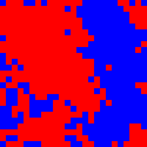
Slo-Gro (slow growth) is a model of a particulate growth process, which happens for example during the aggregation of zinc particles in a two-dimensional film. The ions wander around until they meet the previously settled particles and thus form tree-like structures. DLA stands for diffusion-limited aggregation. The particles settle to form complex, fractal tree-like structures, which remind me of moss, or the Tree of Life - with branches that thrive and branches that wither out (see Fig. 2).

The analogy (well, one of the analogies) for the DLA process presented in the book is simply too precious to pass [1]:

The most colorful (albeit the least realistic) model for a DLA process involves a succesion of drunks wandering about in the dark until they stumble on a crowd of insensate comrades; lulled by the sounds of peaceful snoring, they instantly lie down to sleep. An aerial view of the slumbering crowd by morning light might well reveal the same fractal shape found in a zinc cluster or a soot patch.

On more serious note, the process can be described as follows. The particles (pixels, ions, ...) are initially placed randomly on the circumference of the circle. Each of the particles then wanders randomly (up, left, right, down) until it finds itself in the neighbourhood of some other particle, which is now stationary. The wandering particle then settles down and a now one is launched. The wandering process is stopped when the particles wanders out too far (outside the circle), or if it made too many steps (10 000) without any contact. New particle is generated to replace the strayed one. The process is repeated in a loop. At some point the arena will fill completely, and no new particles will find any more place to join.

In order to make the process quicker, you can influence the Brownian motion of the particles a little. I added a small displacement for the particles at each step, that slowly drags them towards the center, regardless of their random motion. This is controlled by the attraction parameter.

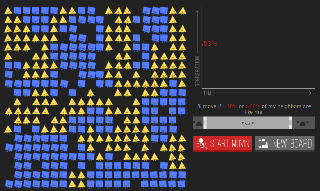
I made a small interactive simulator of the SLO-GRO effect: SLO-GRO Simulator

The code is available here: https://github.com/dagothar/slo-gro (beware: at some points it's one hack upon another!).

In the simulator you can launch your own slow growth process. You can draw on the board to create your own seeds, even during the simulation. You can tweak and mix the colors on the go. The process produces quite interesting graphical results (see figs. 3-9). Make sure to try different values of parameters, as well as different colors.

Fig. 3. The field overgrown.

Fig. 4. Dappled grass.

Fig. 5. Waves of grass.

Fig. 6. Creative palette.

Fig. 7. Delta step overgrown!

Fig. 8. Moon grass.

Fig. 9. Acid eye.

The moss grows quite quickly in the beginning, but it loses its pace abruptly: at some point the growing tree seems almost static. Even though the particles now have smaller distance to travel, more of them is necessary to fill the rings of increasing area (which grows as the square of the distance!). It will take several minutes to fill our Petri dish.

It is interesting to see what is the dimension of the structure generated by the slow growth process. For such a fractal, we can expect its fractal dimension to be somewhere between 1 and 2. Isn't it exciting that there are figures that dwell somewhere between being linear and planar? If you want to learn more about fractals and fractals dimension, I recommend watching an excellent video by 2Blue1Brown.

The fractal dimensions is basically the exponent by which the area of the object increases in response to scaling. For example, the "area" (length) of the line is linearly dependent on its scaling and thus the line is 1-dimensional. The area of a planar figure (e.g. a triangle) raises with the second power of the scaling, and thus the triangle is 2-dimensional. Similarly, a cube is 3-dimensional. The notion of dimension gets complicated with fractals. They tend to have fractional dimensions.

There's an easy way of calculating the fractal dimension of our structure. Simply measure the area (the number of settled points) for several different values of the radius. I did it by letting the moss grow, pausing at certain intervals, and measuring what the radius of the circle containing the sediment is. The data is presented in the plot below (fig. 10).

Fig. 10. Area of the structure vs. the total area.

The fractal dimension is calculated as the slope of the line of the structure area vs the scale plot.  My result is ~1.9. The fractal dimensions cited for Slo-Gro in [1] is 1.58. The discrepancy here is probably due to the attraction parameter; without it the tendrils of the tree tend to be considerably less dense (but then it takes massive amounts of time to generate the data! - see fig. 12). Feel free to experiment.

Fig. 11. Structure area (blue) and the total area (red) in log-log scale. The blue line has slightly smaller slope.

Fig. 12. Sparser structure with the attraction parameter set to 0.1 instead of 0.5.

Literature

[1] A. K. Dewdney, "The Magic Machine. A Handbook of Computer Sorcery", W. H. Freeman and Company, New York, 1990, ISBN: 0-7167-2149-2.

Game of Votes

The Voting Game is a simple model of political process. The game board consists of a grid of squares, each representing a voter of one of two (or several in extended versions of the game) political options (see Fig. 1). The grid is finite, but boundless: it is a surface of a torus. That is to say that the top and bottom edges (as well as left and right) are actually connected.

Fig. 1. The Voting Game simulator.

Each turn, one of the voters is picked at random. The selected voter is influenced in his/hers opinions by the neighbours, and so picks up the colors of one of them chosen at random. Thus, the voter living in a politically uniform area is highly likely to vote the same as his peers. In this mathematical world you can follow a reason in people's opinions, however opportunistic it might be.

The evolution of this system is quite interesting to watch. It seems that once one of the parties develops a numerical advantage large enough, the collapse of the democracy is imminent. It is in fact unavoidable. It might take a surprisingly long time though.

Here you can check the interactive simulator of the Voting Game.
You can generate random distributions of voters in whatever proportion you fancy. You can watch the politics evolve and imagine the governments rise and fall. You can influence voters at a click of the mouse. Live out your political fantasies.

The code is available here.

Fig. 2a. Initial uniform distribution.

Fig. 2b. The distribution after some time.

Mathematical models, regardless how basic, are often very useful and enlightening tools. They let you experience the process as it plays out, and realize that very often the simple rules do not yield simple conclusions. Many people choose to see the world simply laid out; yet the complexity always finds a way to break out.

Please check Vi Harts's wonderful Parable of Polygons if you haven't seen it yet (see Fig. 2). It is a mathematical model in similar vein that illustrates the importance of personal bias in the shaping of the broader societies.

Fig. 3. Vi Hart's Parable of Polygons (from: http://ncase.me/polygons/).

Programming the Wireworld Computer

I previously wrote on Wireworld here: World of wires
It’s an interesting and entertaining cellular automaton, particularly the ease of simulating logic circuits it offers. Please take a look at the text and browse the links provided if you need a refresher on the rules of Wireworld.

One of the most fascinating things ever done in Wireworld is an implementation of a complete working computer (by David Moore,Mark Owen et al.). The computer (and its verbose description) can be found at: https://quinapalus.com/wi-index.html. The computer is presented there running a hard-coded prime search program (by Michael Fryers). Ever since I saw the computer, I thought it would be very fun to have a go at programming it. And wouldn’t it be great to have an interactive online tool to do just that?

The simulator is available here: Wireworld simulator

The program simulates the Quinapalus machine, and provides an interface to inject the instructions/data into its register bank. The machine can then be restarted to run a completely custom program.

The programming of the machine boils down to inserting a proper arrangement of pixels into its general purpose registers. I had to strip down the already working demonstration to revert it to its bare-metal state. In order to do that, I removed every unnecessary electron and synchronized the machine so that the electrons in the registers are aligned. The program can then insert the electrons and tails into the registers at their proper positions. The blank state machine is presented in Fig. 1.

Fig. 1. The blank state of the Quinapalus machine.

The simulation uses my own implementation of Wireworld rules. It’s most certainly not the fastest one available. It is probably possible to save the image generated by the program and import it into the dedicated cellular automaton running software, such as Golly (http://golly.sourceforge.net/). In the future, I’ll think about adding an export feature.

There are also further limitations. It is currently only possible to program the machine using hex codes for the instructions and the data. It would be good to add the possibility of using mnemonics, and - who knows - maybe even a C wrapper? ;)
The memory of the machine is of course limited. Moreover, the program only allows for writing into the registers R1-R52.

I must admit that I am no Javascript wizz. It took me long enough to get the demo working, and the code could arguably use some polish! Here it is: https://github.com/dagothar/wireworld-compiler

If you run into any problems running the code, please let me know. Any suggestions are welcome! I’m looking forward to improve the “compiler”.

(I haven’t probably synchronized the computer completely. Whenever it starts with a new program, it first prints out ‘65535’, then reverts to ‘00000’ before it starts printing out the commanded output. This is perhaps governed by the state of the frequency divisor at the bottom of the unit, but I haven’t yet figured how to set it appropriately.)

Programming the machine

Instruction set for the Wireworld computer is quite short. To be precise, the machine can only execute one instruction:

MOV Rd, Rs                  Move content of register Rs to register Rd

To quote its creators:

We wanted to make the Wireworld computer as simple as we could while still being able to run worthwhile programs. We therefore settled on a highly orthogonal RISC architecture.

The description of the instruction set (repeated below) is available at: https://quinapalus.com/wires10.html

Since only one instruction is available, all the more complicated operations are done using writing to/reading from special purpose registers. These registers are as follows:

Register	Action on read	Action on write
R0	Returns 0	Sends value to display
R53	Returns AND of R54 with NOT R53	Writes value to register
R54	Returns bitwise AND of R53 with NOT R54	Writes value to register
R55	Returns 0	Writes value to register
R56	Returns value in R55 if register R56 is non-zero, and the value in R57 otherwise	Writes value to register
R57	Returns 0	Writes value to register
R58	Returns R58 rotated right one place	Writes value to register
R59	Returns R59 rotated left one place	Writes value to register
R60	Reads value from the register	Writes value to register
R61	Returns sum of R60 and R61	Writes value to register
R62	Returns NOT R62	Writes value to register
R63	Returns program counter value	Causes branch (jump) to the given target

How to arrive at the hexadecimal representation given the mnemonic? Each command consists of two bytes (16 bits altogether). The two bytes contain the address of the destination/source respectively, e.g. MOV R60, R7 translates to 0x3c07 (00111100 00000111 ⇐=> 60, 7).

How to use the simulator?

Simply click ‘Start’ to launch the machine in its current state. The RAM is initially empty, and thus the computer will not do much. Left running on its own, the computer will repeatedly refresh the display with ‘00000’.

You can ‘Stop’ the machine at any time. If you wish, you can ‘Step’ through the simulation manually.

The interface on the left is used for programming the machine. In the text area, enter the hex codes of the instructions (or data) in separate lines. For example:

0x0001
0x0002
...

(Take care, I do not do much validation of the input at this point! If stuff breaks, simply reload the page.)

Click ‘Load’ to load the program into the memory. The machine will be reset and stopped, and you’ll have to ‘Launch’ it again.

Sample program

Now that we have dealt with the boring background, let’s try something practical.
The original program presented on the Quinapalus machine was a prime finder. Let’s try something a bit less sophisticated. How about just counting up (0, 1, 2, …)?

We can do that by writing the following code:

R1    MOV R0, R7    ; send R7 (counter) to the display
R2    MOV R60, R7  ; send counter to R60 (adder input 1)
R3    MOV R61, R8  ; send R8 (1) to adder input 2
R4    MOV R7, R61  ; send the addition result to counter
R5    MOV R63, R9  ; move R9 (R1 address) to jump back to the beginning
R6    MOV R0, R7    ; send counter to display again (branch delay)
R7    0                      ; contains counter
R8    1                      ; 1 for incrementing
R9    1                      ; jump target: R1

Then we have to compile it by hand. The compiled code is:

0x0007
0x3c07
0x3d08
0x073d
0x3f09
0x0007
0x0000
0x0001
0x0001

Go launch the simulator and try to run the program. It will be a while before it counts up a single tick (reserve at least a couple of hours to witness the true glory). The code has room for improvements. See if you can make it run smoother!

Fig. 2. Counter program reaching 2!

​

Burning forests

I think I first encountered the term emergent behaviour in connection with fractals - in a book the title of I have regrettably forgotten.
The very first chapter discussed a phenomenon encountered in a simulation of a simple model of the forest fire.

Imagine the forest as a 2D grid of certain dimensions (let's say it's 100x100). Each of its rectangular tiles represents a small plot of land. On some of these tiles, a tree grows. Some are empty. And - in case of the fire - some host a merrily burning plant.

The rules of the model are as follows. On each turn:

• the empty plot remains empty, 
• a tree starts burning if it has at least one burning neighbour (we use von Neumann neighbourhood, so we only count the tiles which touch the current square on its sides and not the corners),
• otherwise the tree keeps living.

Variations of this model exist (see: https://en.wikipedia.org/wiki/Forest-fire_model). In these, an additional rule often applies: an empty square can in its own time spawn a new tree with a certain chance. Also, random fires can start (e.g. due to lightning strikes).

In our case we are concerned with a more short-term model - that is we do not account for the new growth. Moreover, our fire always starts at one side of the forest. Fig. 1. shows the burning forest.

Fig. 1. Burning forest model. Fire front is visible in red.

The question is: how does the fire front proceed? How many trees does the inferno claim? Surely it must depend on how dense the wood is. It does (see Fig. 2).

Fig. 2. The percentage of the remaining trees as a function of density.

This is where the emergent behaviour occurs. The forest is quite resilient: even with half the squares occupied by the living trees, most of them survive the fire. The things change quite quickly and unexpectedly very soon after the critical density is reached: just short of the 60% mark.

Once the density reaches 60-70% only a few trees ever remain unburned. The numbers of survivors dwindle further towards zero at 80% mark. Uniform front of fire advances on the 100% dense forest.

Where does the number that defines the critical density come from? It's hard to predict just basing on the model rules.

The forest-fire model does not only apply here. Similar approaches are used in the context of disease spread and resistance in populations. In such models, the squares are no longer the trees, but people. Disease replaces the fire. Surely, you can now appreciate the critical impact the vaccinations have on the outcome of epidemies.

I made an interactive tool for you to play with the matches (see Fig. 3). Check it out here: https://rawgit.com/dagothar/burning-forest/master/index.html

Fig. 3. Burning forest simulator.

You can check the code out here: https://github.com/dagothar/burning-forest

Throwing Pi

It’s a Pi day!*

It is possible to calculate using nothing more elaborate than a dart board (and a couple of darts). Throwing darts at the circular target drawn on the board, we can take note how many hits did in fact fall within the circle, and how many hit the bounding box of the circle.

Since the area of the circle inscribed inside a square is of that of the square, we can easily calculate based on the number of hits and misses:

Of course, this is a game invented for mathematicians, who can boast -among other things - of true randomness in their dart game. Being random is surprisingly hard for regular humans.

I made a little interactive gadget to simulate calculating using the dart board: https://rawgit.com/dagothar/pi-throw/master/index.html

Fig. 1. Throwing Pi.

You can now try your hand at the game. Simply click on the board to place the dart. You can make the computer throw the dart for you by clicking on Step. You can also launch a whole series using Start/Stop.

The method does not converge very quickly, and is prone to being slightly wrong about . You can help it to get the right result by placing the darts as it goes.

* At least in the uncivilized part of the world, where they put their months in front of the days: 3/14. We can’t have the day the other way around though - could it be that they are right?

​

Langton's Ant

Langton's ant is a small bug that crawls tirelessly on a floor tiled with rectangular plates, which are black on one side and white on the other. Whenever the ant first steps on the plate, it checks its color and changes direction:

• if the plate is black - it turns to the right,
• if the plate is white - it turns to the left.

It then proceeds - a nasty little vandal - to turn over the plate it is now standing on: white to black or black to white. And then it moves forward (in the new direction) again.

Could the rules be any simpler? Of course, with such simple rules we do not expect the ant to exhibit any interesting behaviour. It will probably just run around in a circle, and maybe flip some tiles randomly. Nothing interesting can come out of such a system. Or can it?

Let's see what happens anyway. At first, it seems our predictions were correct. The ant produces simple and symmetric patterns (see Fig. 1).

Fig. 1. At first nothing interesting happens.

After a couple hundred of iterations, the patterns seem still quite symmetric and predictable (see Fig. 2).

Fig. 2. Making nice patterns.

After 2000 iterations chaos emerges (see Fig. 3):

Fig.3. The beginning of chaos.

We now change our prediction. The ant is going to fool around and paint the whole floor with no regard to symmetry or aesthetics - it is going to be a pure chaos.

Let's watch a little more...

This is what happens after ~11,000 iterations (Fig. 4):

Fig. 4. The ant escapes, leaving a "rose" behind.

After tumultous youth, the ant has abandoned its chaotic ways and started behaving orderly. The structure left behind reminds me vaguely of a rose. The ant now constructs a "highway", taking 104 steps to make yet another turn in the coil of the stalk.

How did this happen? Why did such simple rules result in so many different kinds of behaviours? From order, to chaos, to order again. How did the number 104 come up from the rules we have defined in the beginning?

There was certainly no way to predict the final result from those.

You can play with the Langton's ant using the simulator I made: https://rawgit.com/dagothar/langton-ant-js/master/index.html

As usual, the source files are provided: https://github.com/dagothar/langton-ant-js

 

Simply click Start. You can also try to make the ant go step-by-step with the aptly named Step button.

You can also draw on the board with the mouse! What do you think will happen when the ant encounters your drawings? Can you trap it? Will the ant draw a different shape?

 You can read more about the Langton's ant here: https://en.wikipedia.org/wiki/Langton's_ant

Modelling pendulum

Erratum: I have now fixed the errors that were present in the calculations in the previous version of the post.

This term I am teaching a course on modelling dynamical systems. In this post I will present a simple example of modelling a cart-pendulum system (see Fig. 1).

Fig. 1. A cart-pendulum system.

The system consists of a pendulum mounted on a cart sliding horizontally. The pendulum is assumed to be a point mass hanging on a massless wire at an angle of θ The cart is pushed by some external force u=f(t) and its position is defined as z The following parameters define the properties of the system:mass of the cart m1, mass of the pendulum m2 and the length of the pendulum l.

The problem is formulated as follows. Find the equations of motion for the system using Lagrange equations. Linearize the non-linear model obtained. Observe and compare the behaviour of both the linear and the non-linear models.

We will solve it in the following steps:
1) How many degrees of freedom (DoF) do we have here?
2) What form of Lagrange equations should we use?
3) What’s the kinetic energy (K) and the potential energy (U) of the system?
4) Solve Lagrange equations.
5) Define state-space non-linear model.
6) Linearize the model.
7) Simulate the behaviour of the models using Matlab.

Let’s go!

1) First, it is quite obvious that the system has two degrees of freedom: z and θ.
It ought to be said that there are several ways these generalized coordinates can be chosen, but this is the most convenient choice in this problem.

2) The Lagrange equations for this system are going to be in the following form:

3) Since the Lagrangian of the system is defined as its kinetic energy K minus its potential energy U, we have to find out what K and U are. There are two bodies in the system that have masses (m1 and m2). K will therefore be:

We have to be careful while calculating velocities v1 and v2. The velocity v1 is straightforward, but v2 consists of the carrying linear motion of the cart plus the motion of the pendulum relative to the cart. Moreover, the velocity of the pendulum around the cart can be split into two orthogonal vectors: and .

Since and are calculated as follows:

The will be:

The kinetic energy K will therefore be:

The potential energy U is associated with the mass of the pendulum m2 hanging in the gravitational field. Here, we are going to introduce temporary variable y which describes the vertical displacement of the pendulum:

4) Having calculated both K and U, we can formulate the Lagrangian:

In order to solve the equation, we have to calculate these pesky partial derivatives - first for z, and then for θ. I did this in WolframAlpha.

Now, subsituting the derivatives and the generalized force u into the Lagrange equations, we get a system:

We are not going to calculate this by hand. I have used the following WolframAlpha query (and then substituted the names of variables back):

solve for x, y: (m+n)x+nl(ycos(f)-w^2sin(f))=u, xlcos(f)+yl^2+glsin(f)=0

The equations of motion are:

5) We can now construct the (non-linear) state-space model. This is done by first naming the state-space variables:

and then substituting into the equations above:

This non-linear system is of form:

where, for instance:

6) Linearization of the system is done by replacing the non-linear functions with their first-order approximations at selected “operating point”. Mathematically this is one by assuming the following linear model:

The Δx, Δu and Δy are defined as offsets from the operating point:

Let’s define our operating point as:

The matrices A, B, C and D are calculated as:

It isn’t as scary as it looks. just says that we have to calculate the derivatives of functions , and so on partially over , etc. and put them into the matrix A. The says: after calculating the derivative, substitute and (assumed previously) into the equation.

I have used the following WolframAlpha queries to compute the (non-trivial) derivatives A23, A24 and A43, A44:

d/dx (nsin(x)(gcos(x)+ld^2)+u)/(-ncos(x)^2+m+n)

d/dy (nsin(x)(gcos(x)+ly^2)+u)/(-ncos(x)^2+m+n)

d/dx -(gsin(x)(m+n)+cos(x)(lnd^2sin(x)+u))/(l(-ncos(x)^2+m+n))

d/dy -(gsin(x)(m+n)+cos(x)(lny^2sin(x)+u))/(l(-ncos(x)^2+m+n))

Similarly, B would be:

In order to observe all state variables, define C = I. D has to be filled with zeros, with dimensions that agree with B and C.

7) We can now see how these work!
The scripts for this problem can be found at: https://github.com/dagothar/mos03

By default, they generate the object response with u=0, but with a starting condition in which the pendulum starts at a positive angle to the vertical. And here are the results:

Fig. 2. Reponse of the non-linear system (to the left) and of the linearized system (to the right).

The responses seem very similar when a small initial angle displacement is given. Things change when the pendulum is placed at a larger starting angle.
Can you guess what happens?

​