Airfight

Long time ago (almost 20 years!), when I was a brilliant young lad who still knew pretty much everything and was consequently tremendously bored sitting through the classes, I invented a simple pen-and-paper game to play with my friends.

Airfight (Samoloty) is a turn-based WWI / WWII airplane duelling game that can be played with only a piece of paper, a pen or two and any straight-edge implement. It greatly resembles the way that miniature battle games are played nowadays, but I haven't yet heard of any of them when I first made it up.

Was the game, fun, playable and addictive? Well, let me just say that it had easily been more attractive than the long and interesting hours of religious studies! I also managed to get a couple of people to play it, so it couldn't have been half bad ;)

Let me quickly take you through how the game was played (as far as I can recall the rules).

Fig. 1. I also made a PC implementation - more on that below.

THE RULES

The purpose of the game is to win an airplane duel. Each player controls one of the airplanes and they act in alternating turns. The fight is won when the opponent's aircraft crashes or its pilots are killed. You can force the crashing of the plane by destroying it with your guns directly, damaging it so it loses all its fuel, engine power or steering. When the steering is destroyed, the plane will often crash on the page's border.

The game was meant to be very simple and require little in the way of accessories to play it. As a consequence, some of the rules (like hit zones and the turning radius) are quite arbitrary. Perhaps they could be improved somehow?

Setup

To play the game you need: a piece of paper (usually A5, but any larger size is also alright), a pen (two if you do mind sharing) and any straight edge implement (a ruler is good). Each player draws his airplane doll and picks a starting position on the opposite sides of the page. The typical setup looks like this:

Fig. 2. Game setup.

Airplane systems

The airplane doll is used to track the damage done to the aircraft and the amount of remaining fuel and ammo. The game uses a clever (even if I say so myself!) mechanic to establish the hit zones with damage to different systems affecting the performance of the plane in different areas. The plane doll looks like this:

Fig. 3. Airplane doll.

The round circles indicate the damage done / remaining hit points of the system. An empty circle is 3 HP (or 0 damage), while a completely shaded circle is 0 HP (or: completely destroyed). Some systems have more than one circle to represent its health.

Fig. 4. Representing hit points / damage. Top row illustrates a typical system. Bottom row illustrates the damage to the engine block.

The systems of the aircraft are:

• Propeller, which is used to move the aircraft forward. The propeller is fragile (3 HP) but it is a relatively small target. When the propeller is completely destroyed, the airplane loses 1 speed per turn. When the plane loses all its speed it  crashes.
• Engine. The engine provides power to the aircraft. Each turn you can only move the plane by as many squares as the engine HP left (which is 6 squares at the beginning). When the engine is destroyed, the plane crashes.
• Oil (coolant). This serves as a shield to the engine. Typically, the enemy bullets would first damage the coolant, only to be able to hit the engine after no oil is left. After the oil reservoir is first hit, it springs a leak, and from that point on it loses 1 HP/turn. While the leak is going, the aircraft leaves a dense smoke trail. (Optional: after the oil is all gone, the engine loses 1 HP/turn as well.) There are 4 circles for the coolant, and so the system packs 12 HP.
• Crew. The crew resides in the cockpit in the very center of the craft. It would rarely get hit (you have to be very persuasive as the determination of hit zones is quite arbitrary!), but once the pilot dies, the player loses. The crew has 6 HP.
• Guns/ammo. The plane has two guns, each with it's own supply of ammo (4 circles per gun, or 12 HP - or shots). Each shot taken with a gun reduces the supply by 1 HP. Any hits to the ammo zone also reduce the amount of shots left appropriately.
• Fuel. The fuel forms the biggest hit zone. Each turn you lose 1 HP of fuel for movement. Each hit to the tank also destroys the fuel left by appropriate amount. When the tank is struck, a leak forms, which then empties the reservoir at the rate of 1 HP per turn. Once the fuel is fully depleted, the plane starts to lose 1 speed per turn, and when it reaches 0 it crashes. The plane with a leaking tank leaves a trail of smoke. Each plane starts with 18 HP worth of fuel, but you can customize that amount.
• Left/right steering. This is split left to right and into the tail/wing assemblies. Each side has 6 HP. The damage to the steering surfaces affects the controllability of the craft (more on this in the following section).

Flying

During your turn you can execute two actions, one after another: moving and shooting. I think in the original game it was always 'move first, then shoot', but I see no reason why the sequence of the actions can't be picked by the player.

There are two parts to the movement: speed and turning radius. The first is controlled by the remaining engine HP left, in that you can only move as many squares as the engine HP left. You can move on any sort of curve and it's the length of that curve that counts. You have to do your best to approximate the distance.

Fig. 5. Flying the plane with various levels of speed.

The turning radius decides on the maneuverability of the plane. You have two sets of steering controls, each of which can be damaged or destroyed and you can only turn left/right as much as the remaining health of the system lets you. This is still pretty much arbitrary (modern figure games use curve shaped accessories to determine the turning radius rigorously), but you'd have to do your best to fly your plane true to its current capabilities. For instance, with the right side rudders completely destroyed, you shouldn't be able to turn right at all!

You have 6 HP for the steering on each side (12 HP in total). The turning radius could be scaled with the current HP to total HP ratio using this picture for reference:

Fig. 6. Turning radius related to the steering HP left.

Shooting

When you choose to shoot, you can use each of your guns once. There is an arcade aspect to this mechanic. You place a dot 1 square away from where the gun is on your plane avatar (it's either left or right bottom corner of the triangle) and use the ruler to draw a straight line through those two points. You can only shoot vaguely in 90 degree sector facing front of your plane.

Fig. 7. Shooting the target.

A hit is scored when the line crosses the enemy's avatar. You have to use the plane doll to approximate where on the enemy craft the hit has occured and process the damage accordingly:

Fig. 8. Finding out where the damage occured.

There is a social aspect to this, as the hit zone assingment is quite arbitrary. Arguing is allowed, provided you do it in a civilized way. Maybe a good way to keep it fair would be that both you and your opponent each decide on the hit zone and then you use a coin toss to pick one?

Each hit takes out 1 HP of the affected system, but you can use a damage multiplier (e.g. 2x) if you wish for a shorter game.

Sample game

Ok, let's try with a sample game!

Fig. 9. Player at the bottom wins. The plane on the top crashes due to the lack of fuel and due to oil leak destroying the engine.

I found my old notebook in which I apparently play-tested the game:

Fig. 10. Old game of  Samoloty.

AIRFIGHT ON A PC

Much, much later (but still like ~10 years ago), I made a computer implementation of the game.

It was done in C++ and used the Allegro library (http://liballeg.org/) for graphics and control. I used soe of the graphics I found on the web for the planes and the backgrounds and to my eternal shame I didn't record the authors (if you know them, please let me know).

The game is available on my GitHub HERE. Binaries are included, so all you have to do is to download the game and play.

Fig. 11. Game menu.

Features

• Two-player split-screen real-time shooting match!
• Several aircraft to choose from (Spitfire, Bf110, Flying Fortress and F16),
• Different types of weapons (machine guns, flak cannons, rockets, self-aiming guns, bombs),
• Hit zones,
• Very primitive artifical "intelligence".

Installation

As mentioned above, simply go to my GitHub repository and download the game. The binaries for Windows are included. If you wish, you can build the game from the source. A Code::Blocks project for the Windows version is included, and a Linux Makefile is also available.

For the Linux version, you will have to install the Allegro library package (version 4.2).

Playing the game

Select your starting craft and start a new game! If you wish to play with another person, you should first disable a primitive form of artificial intelligence enabled by default for the second plane. Go to the Options and switch off the Test2 checkbox.

The controls are as follows.

Player #1:

• ← → turn the plane left and right,
• ↑ accelerates the plane,
• ↓ switches the boost on and off (the boost briefly multiplies your speed),
• Right Shift cycles between the weapons,
• Right Control fires the guns.

Player #2:

• Z C turn the plane left and right,
• X accelerates the plane,
• A switches the boost on and off (the boost briefly multiplies your speed),
• Left Shift cycles between the weapons,
• Left Control fires the guns.

Just the same as in the pen-and-paper version, your goal is to destroy the opponent's plane. There is a brief warm-up period at the start of the game during which your weapons are locked. Once you achieve a certain speed, your plane 'takes off'. From that point you can't slow down too much, otherwise you'll stall and crash.

There are hit zones here as well. Destroying your engine will make your plane slow down and stall. Fuel may leak, the ammo may get destroyed and the guns may jam. The hit zones are implemented through an underlying sprite map with color encoding:

Fig. 12. Hit zones of the flying fortress.

The bullets each cover some distance between frames and so there is a chance for them to hit even the internal aircraft systems by chance.

Fig. 13. Flying Spitfire.

Fig. 14. Flying Bf110.

The game isn't terribly well balanced. Who knows, maybe I'll make a new version some day.

As to why do the planes seem to fly belly-up in the sky... You won't understand ;)

Making Deventer's Mazes

In my previous post (the very first one!) I described how to solve an unique 3D maze puzzle by using RRT path planner provided by RobWorkStudio.

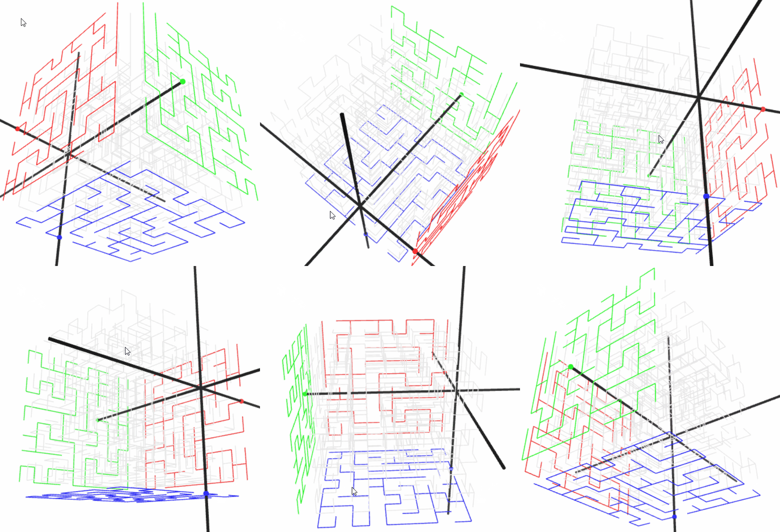
The original puzzle was designed by Oscar van Deventer and it consists of three orthogonal flat plates, each carved with the 2-dimensional maze. The three plates restrict the movement of a star-shaped cursor within the cube, such that it can only move on an invisible 3-dimensional path projected by the mazes on the side (see fig. 1).

Fig. 1. Deventer's maze recreation. The cursor is the star-shaped orange-ish shape inside the cube.

We were left with an open question of how to programmatically generate a new puzzle just like this.

The naive extension of backtracking algorithm into 3D works well, but it is not suitable to make Deventer's Maze without modification. The projection of 3D path generated by the algorithm on the orthogonal walls of the puzzle would inevitably contain loops. Indeed, the absence of loops on the walls seem to be the leading constraint in this problem.

A simple idea would be to build 4 separate mazes in parallel using the backtracking algorithm. 3 of these mazes would be two dimensional, representing the sides of the cube, while the fourth one would be fully 3D. The 3D maze would be the primary one used for the construction: the backtracker would explore the cells at will, except that while finding neighbouring adjacent unvisited cells, the side mazes would be used to guard against forming loops. Simply put, if the new candidate unvisited cell's projection is visited, and  no direct connection exists to that cell on the side maze, it is not elligible to be the candidate for the neighbour. Unvisited projection cells and those that already have connection (including to itself) are allowed.

This generation procedure has to be repeated, since not all of the cells will be visited on the first call of the backtracker. Some of the cells will be inaccessible from any one given path, and thus the backtracker has to be called again, starting from the next unvisited cell found.

This is perhaps a little obfuscated explanation; please check the code for the details.

I made an implementation of the Deventer Maze generator in Javascript HERE.

The repository is available at: https://github.com/dagothar/deventer.

.

Fig. 2. JS implementation of the generator. Take a look!

This is how the algorithm looks in action (fig. 3):

Fig. 3. Generating a new 8 x 8 x 8 maze.

The result is presented below (fig. 4):

Fig. 4. The result.

Of course, it is also possible to build larger puzzles (see fig. 5), although it quickly becomes a computational challenge.

Fig. 5. Generating large mazes may take a while (25 x 25 x 25).

I programed the generator such that you can try solving the generated mazes as well. The black star shape is the cursor, and you can move it using the W / A / S / D / Q / E keys:

• W / S move the cursor in the X direction (away / towards the red maze),
• A / D move the cursor left / right (away / towards the green maze),
• Q / E move the cursor down / up (towards / away the blue maze).

It is quite difficult to solve even the simplest mazes (see 3 x 3 x 3 in fig. 6)! In case you get stuck, you can use the input fields for the cursor position in the panel on the right to move without the path constraints.

Fig. 6. Navigating the 3 x 3 x 3 maze.

The panel on the right also provides some information. First, it indicates if the current maze corners all belong to a single path component. This will not always be the case. Next, the number of separate paths is provided. The first path will most likely be the largest component and its size is also provided.

There are still a couple of problems with this approach though. Very often, no path is generated that connects all corners of the maze. Such a result I do not consider to be a proper puzzle, since not all of the corners can be reached from single chosen starting configuration. The issue could perhaps be amended by growing separate and unbiased trees at every corner of the cube and then prioritizing the merging of the trees. I am not sure that would guarantee that the generated puzzle is proper.

Of course, it is likely not possible to make a nice random and aesthetic tree exploring all cells of the puzzle. The original creation itself did have cells which were not reachable from the starting configuration.

It would be nice to create the actual 3D models based on the generator presented here. I will work on that in the future.

Chaos game

This post is inspired by the Numberphile video I watched recently: https://www.youtube.com/watch?v=kbKtFN71Lfs.
I greatly recommend watching it and subscribing the channel if you haven't yet done so - it's full of all sorts of mathematical goodness for the mathematical geek in you.

I made an interactive JavaScript implementation of the game, which you can check out HERE (see fig. 1).

The code for the demo is available on GitHub: https://github.com/dagothar/chaos-game. Let me know if you spot any bugs!

Fig. 1. Chaos game demonstration.

So, what is the Chaos Game?
 It's a method for creating fractals. You start with a blank page, a set of vertices arranged in a polygon and a randomly selected starting point. Each turn you select one of the vertices of the polygon and travel towards it covering a certain portion of the distance (for example 1/2 - it is also the same each turn). You draw a dot each time you stop to pick another vertex to travel to. The procedure, simple enough as it sounds, yields some surprisingly complex results.
With a starting set of vertices arranged in a triangle, and covering half the distance to the randomly selected vertex each time, a Sierpiński triangle emerges (see fig. 2).

Fig. 2. Sierpiński triangle is made on a triangular grid with the step parameter set to 0.5.

 More complicated setups yield deservedly rewarding fruits (see fig. 3).

Fig. 3. Pentagonal fractal with step=0.67.

A very curious thing happens when a portion of the game board is barred against the intrusion of the randomly wandering point. In that case, the shape of the restricted area is repeated fractalised all over the board in form of the areas untouched by the point iterations (see fig. 4). The figure shows the blog icon repeated within a square setup of control points. Is it possible to do the same inside a triangle or a pentagon? Does the step size parameter has to be changed?

Fig. 4. DeltaStep logo fractalised in a square after 100,000 iterations.

How to use the demo?

Simply click Start. The game will be played automatically between the vertices of the polygon specified by the red dots. You can Pause the game at any time.

Clear removes the dots, but not the vertices. You can also Download the currently generated image yo your computer.

The Step size slider controls the distance which is covered towards the next randomly selected vertex each iteration (0.0 to 1.0).

You can control the speed at which the new dots are generated. By default, the callback is invoked every 1 ms, but that speed is mostly likely limited by your hardware. You can slow the game down up to 1 dot/sec by using the slider.

You can also customize the colors and the dot size.

Controlling the control points. You can move the control points by hovering over them, clicking and dragging them around. To remove the control point, simply drag it outside the board.

You can add new control points by clicking the Add new point button on the left side of the interface. The new point is placed in the middle of the board, from where you can drag it to wherever you like.

You can make any regular polygon setups by using the Make n-gon button. The number on the right of the button controls the number of the regular polygon vertices.

Defining the restricted area. You can paint on the board with your mouse. Simply click and drag around outside the control points. The painted area will be blocked for the game iterations, thus allowing you to create the fractals of custom patterns. (Note: do not block too much of the board - the script may get stuck trying to find a new possible jump target).

There are several unanswered questions the game leaves us with. What happens when the control points are placed on the vertices of a concave polygon? What if the polygon is distorted? What does the step size actually do? How do you achieve the fractalisation effect with more or less points than four?

The chaos game invites.

Literature

[1] Numberphile, Chaos game video, available: https://www.youtube.com/watch?v=kbKtFN71Lfs

[2] Wikipedia,  Chaos game, available online: https://en.wikipedia.org/wiki/Chaos_game

Upside down

It is intuitive to expect that after releasing a raised pendulum it will tend to swing around and eventually stop at rest at the bottom. It is perfectly reasonable: after all the gravity acts downwards, and the loss of energy due to friction will slowly bring the movement to stop. Of course, you can also balance the pendulum upside down, but it is not a stable configuration - any slightest disturbance will topple the system.

Situation changes when you introduce vibrations while holding the pendulum. The oscillation fools the pendulum, as if confusing it to where the top and where the bottom is. The shape of the potential function changes and new stable minima appear. You can now easily balance the pendulum upside down! In fact, it is possible to balance the pendulum at any angle to the vertical. (You can’t do it by hand. The required amplitude and the frequency of oscillations are too big to be generated this way).

It’s a very curious phenomenon, and I’m very grateful to my friend Maciej Ciężkowski who drew my attention towards it. The inverted pendulum is one of his areas of research, and he’s done some great work pursuing that interest. I encourage you to check out his papers ([1, 2]) which explain in detail the things you’ll read about below.

I wanted to observe what exactly is happening when you subject the pendulum to oscillations - and what better (and cheaper!) way to do it if not to make a simulation?

(One more note: this is open-loop control, so no feedback is used.)

Pendulum simulator

The interactive demonstration of the phenomenon is available HERE.

The source code is hosted at GitHub: .https://github.com/dagothar/inverted-pendulum

Fig. 1. Pendulum simulator.

Features:

• pendulum dynamics simulator,
• completely parametrizable,
• introduce pendulum base oscillations,
• measure pendulum angle and angular velocity,
• measure pendulum angle with vibrations filtered out,
• observe the shape of gravitational potential Ug and the effective potential Uef,
• slow-mo,
• click to drag pendulum around,
• bugs (?).

The pendulum is shown in the middle (it’s the black rod with a black circle on its end). The base of the pendulum is shaken by a linear actuator (black rectangle). The angle of the actuator (the plane of oscillations) is shown as the dashed black line denoted β. Thin dashed black line shows the current angle of the pendulum θ. The blue line shows the angle of the pendulum ψ after filtering out the quick vibrations (which are due to the shaking).

The pendulum is surrounded with a plot shown in polar coordinates. The green line shows the potential due to gravity Ug, while the red line shows the potential modified due to oscillations Uef. It is somehow tricky to spot the minima and the maxima of a function plotted in polar coordinates. The grey concentric circles represent the different levels of the potential and the dashed red circle shows the value of the potential at the current position of the pendulum.

The panel on the left allows for the modification of the parameters. You can restore the default values by clicking the Reset parameters button at the bottom. The panel on the top right contains a set of controls. Here you can Reset the system, Start and Pause the simulation and tweak the inputs. I suggest to begin with changing the plane of the oscillations β (don’t do it too quickly!). You can slow down the time by using the Time scale slider.

You can also interact with the pendulum directly. Simply click on the image in the center. In the paused mode, the pendulum will be placed wherever you have clicked. In the running mode, a force will be added to the pendulum that will attract it to the cursor’s location.

There was a lot of trickery and fiddling required to make this work (wrap-around issues and frequency scaling were particularly nasty). Do not hesitate to ask about the technical details.

The model and the parameters will be described in more detail below.

The model of the pendulum

The model of the pendulum is presented in fig. 2.

Fig. 2. The model of the pendulum.

The pendulum consists of a rod of length l and mass m, mounted on a linear actuator of length 2A. The rod has uniform density. The angle of the pendulum from the vertical is denoted θ. The angle of the oscillation plane is
β. The linear actuator induces oscillations of frequency ω. The position of the center of mass of the pendulum is (cx, cy), while the position of oscillating hinge is (rx, ry). The gravitational acceleration g acts downwards.

The parameters are described in the following table.

#	parameter	units	description
1	θ0	[rad]	the initial angle of the pendulum
2	dθ0	[rad/s]	the initial angular velocity of the pendulum
3	m	[kg]	the mass of the pendulum
4	l	[m]	the length of the pendulum
5	g	[m/s^2]	the gravitational acceleration
6	Amax	[m]	maximum amplitude of the oscillations (scales the amplitude slider)
7	ωmax	[rad/s]	maximum frequency of the oscillations (scales the frequency slider)
8	dmax	[Ns]	maximum damping for the pendulum (scales the damping slider)
9	kpull	[Nm]	spring coefficient for pulling the pendulum with the mouse
10	dpull	[Ns]	damping coefficient for pulling the pendulum with the mouse
11	kψ	[1]	low-pass filter coefficient k for the filtered pendulum angle ψ
12	Tψ	[1]	low-pass filter coefficient T for the filtered pendulum angle ψ

The equations of motion

The dynamics of the pendulum are described by the following equation:

One might also add a damping term to curb the oscillations, like so:

It is also necessary to calculate the position of the base point of the pendulum (the one driven by the oscillations):

It’s quite easy to derive these equations through Lagrangian formalism. Start with the equations of motion for the oscillating base, then add the rotational swing of the pendulum for the velocity and the position of the center of mass of the pendulum. These expressions can then be plugged into potential and kinetic energy calculations, which make up the Lagrangian: L = T - U.

The equations of motion pop out from:

The filtered angle of the pendulum is computed with the use of a low-pass filter to cut out the high frequency oscillations. The filter equation is:

(This filter could use some tuning perhaps.)

The effective potential

What makes the pendulum think it should go to a certain position is the force due to the gradient of the effective potential. This is the potential felt by the slowest mode of the pendulum oscillations. The effective potential Uef is calculated as follows [1]:

Examples

With no oscillations introduced, the pendulum behaves as expected: it falls down from its top unstable position and slows down at the bottom (see fig. 3).

Fig. 3. The pendulum falls down when no oscillations are present.

The effective potential changes its shape when the oscillations are introduced. The fig. 4 shows the pendulum oscillating around a new stable point at 45 degrees from the vertical. Notice how the minimum is visible in the shape of the Uef function: the red line rises on both sides around the pendulum position and the tangent red dashed circle.
You might notice that you have to place the plane of oscillations somewhat “higher” than the desired angle of the pendulum. You can find the formula for this angle in [1].

Fig. 4. Pendulum balanced around 45 degrees to the vertical (default parameters; β=0.591).

But how to achieve that stable configuration? The fig. 5 shows the pendulum moved into its top position by first introducing the oscillations and then rotating the plane of the vibration. Notice how the shape of the effective potential deviates from the base as the frequency of the oscillations is increased.

Fig. 5. Stabilizing the pendulum in its top position.

There are still some open questions here to answer. How to achieve the time optimal transit between the positions? Is it possible to arbitrarily shape the potential function? What on Earth can this be used for?

Literature

[1] M. Ciężkowski, Stabilization of Pendulum in Various Inclinations Using Open-Loop Control, Acta Mechanica et Automatica. 5(4), 22–28 (2011), full text available: http://www.actawm.pb.edu.pl/volume/vol5no4/CIEZKOWSKI_EN_2011_105.pdf
[2] M. Ciężkowski, Dynamic stabilization of the pendulum in a moving potential well, 2016 21st International Conference on Methods and Models in Automation and Robotics (MMAR), Miedzyzdroje, 2016, pp. 54-58. doi: 10.1109/MMAR.2016.7575087

​