Double pendulum

Introduction

It seems like it's breaking the laws of physics... and certainly the laws of our intuition! Certainly, the movement of the chaotic pendulum just looks wrong. And how come such a simple physical system exhibits such a vivid variety of behaviours?

A double pendulum is simply two rods attached together. You release it from a certain height and the rods twist and turn together (see fig. 1). It is not just an artifact of simulation - the real device behaves just like that (watch it here  for example, narrated by Steve Mould).

Fig. 1. Chaotic dance of the double pendulum.

The double pendulum is a chaotic system. The evolution of its parameters in time is very sensitive to the starting configuration. If you release it the from a position just a few milimeters off, it will move completely different than in the previous experiment. In making this demonstration I wanted to show this intriguing behaviour.

Simulator

The JavaScript interactive demonstration of the double pendulum (see fig. 2) is available here: DEMO.

The source is available on GitHub: SOURCE.

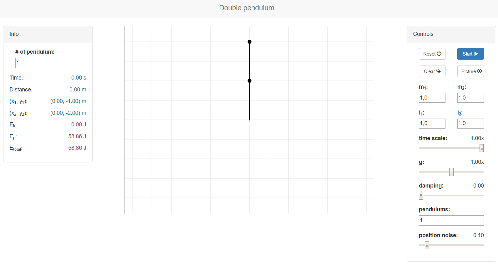Fig. 2. Double pendulum JavaScript demonstration.

So what are the features?

• simulate double pendulum with custom parameters (masses, lengths, time scale, gravitation),
• click on the image to place the pendulum,
• watch beautiful trails!,
• observe positions and energies in the panel on the left,
• add multiple pendulums with a slighly varied initial position to see the effects of chaos,
• QWOP style force control!

Click Start/Stop to see the simulation going. You can place the pendulum wherever you want by simply clicking in the animation. I made the inverse kinematics solver try to place the pendulum with the 'elbow' pointing downwards at any position.

The color of the trail is going to be randomly generated every time you click. The parameters can be changed in the panel on the right at any time.

You can slow down the animation and add some damping so that the pendulum will eventually stop. The damping force is proportional to the angular velocities of the two rods.

You can add multiple shadows of the original pendulum by changing the value in the pendulums box. The new pensulums will be added close to the current position of the pendulum with a certain level of uncertainty, which you can control by the position noise slider. The noise is generated as offsets in the rod angles.

You can control the pendulum manually as well. I implemented QWOP style controls (see fig. 3):

• Q accelerates the top rod clockwise,
• W accelerates the top rod counterclockwise,
• O accelerates the bottom rod clockwise,
• P accelerates the bottom rod counterclockwise.

Fig. 3. Moving the pendulum QWOP style.

Model

Double pendulum is a deceptively simple physical system. It should be relatively simple to derive the equations of motion through the Lagrangian formalism; the equations get complex very fast though. I quickly gave up trying to do this on paper and enlisted help of Matlab. Matlab in turn proved to have problems with symbolic expression derivatives wrt. to other symbolic functions... I ended up manually substituting some of the equations. The physical model of the contraption is shown in fig. 4.

Fig. 4. Physical model of a double pendulum system.

The model is described with the following properties:

• θ1, θ2 - angles of the pendulum rods relative to the vertical,
• l1, l2 - lengths of the rods,
• m1, m2 - masses at the ends of the rods,
• τ1, τ2 - additional torques at the pendulum joints,
• g - the gravitational acceleration,
• b - damping coefficient.

There seem to be lots of sources available on the web for the double pendulum. I checked some more popular Google results, and only one of those was correct (check the page out, they also have a nice interactive demo going!): https://www.myphysicslab.com/pendulum/double-pendulum/double-pendulum-en.html.

I wanted to have a slightly extended model, allowing for introducing user input torques in the pendulum joints, and including a simpel damping model. I used the following script to obtain the equations of motion (see fig. 5): SCRIPT.

Fig. 5. Equations of motion of the double pendulum system (click to enlarge).

And this is the LaTeX source for your convenience: LATEX.

The equations of motion are solved in JS using a Runge-Kutta 4th order fixed step solver (dt = 0.01 s).

Inverse kinematics

One of the features of the simulator is moving the pendulum to the cursor position with a mouse click. This requires a method for converting the (x, y) coordinates to the proper values for the pendulum joints (θ1, θ2). A simple way to tackle this is to use transposed Jacobian to iterate to the correct solution.

The position of the bottom bob of the pendulum is given by:

The Jacobian describes how the (x, y) changes due to changes in (θ1, θ2):

This is calculated as:

The following algorithm is executed then:

1. Assume a starting configuration (θ1, θ2).
2. Find the position of the pendulum (x, y) = f(θ1, θ2) at the assumed configuration.
3. Calculate the error vector e = (xdesired, ydesired) - (x, y).
4. If the magnitude of the error vector is sufficiently small (|e| < ε) finish.
5. Calculate the Jacobian J, and transpose J'.
6. Compute the offset to the (θ1, θ2) coordinates: Δθ = J' e.
7. Update the θ coordinates: θ = θ + α Δθ.
8. Go to step 2.

Examples

Some examples generated with the demo tool are presented below.

The first GIF shows the chaotic behaviour of the system. Two pendulums are released close together:

Fig. 6. Two pendulums start close together but soon grow apart...

Fig. 7. A bowl of pendula seems to be a proper collective noun.

You can add up to 100 pendulums (see fig. 8)!

Fig. 8. Uh-oh...

And this is what happens when you spin them around (and l2  is smaller than l1):

Fig. 9. Pendulum doughnut.

I wish I could add all the GIFs here! The generated images are massive though, so you'll have to check out the simulator yourself ;)